概要信息：

1
Kinetic Rate in a PFR Reactor:  HYSYS 
By Robert P. Hesketh  Spring 2002 
 
In this session you will learn how to install a tubular reactor in HYSYS with a kinetic reaction 
rate.  This HYSYS reaction rate will allow specification of an irreversible reaction.  We will 
ignore equilibrium in this tutorial. 
 
The references for this section are taken from the 2 HYSYS manuals: 
Simulation Basis:  Chapter 4 Reactions 
Steady-State Modeling:  Chapter 9 Reactors 
 
Reactors. 
Taken from:  9.7 Plug Flow Reactor (PFR) Property View 
 
The PFR (Plug Flow Reactor, or Tubular Reactor) generally consists of a bank of cylindrical 
pipes or tubes. The flow field is modeled as plug flow, implying that the stream is radially 
isotropic (without mass or energy gradients). This also implies that axial mixing is negligible.  
 
As the reactants flow the length of the reactor, they are continually consumed, hence, there will 
be an axial variation in concentration. Since reaction rate is a function of concentration, the 
reaction rate will also vary axially (except for zero-order reactions). 
 
To obtain the solution for the PFR (axial profiles of compositions, temperature, etc.), the reactor 
is divided into several subvolumes. Within each subvolume, the reaction rate is considered to be 
spatially uniform. 
 
You may add a Reaction Set to the PFR on the Reactions tab. Note that only Kinetic, 
Heterogeneous Catalytic and Simple Rate reactions are allowed in the PFR. 
 
Reaction Sets (portions from Simulation Basis:  Chapter 4 Reactions) 
Reactions within HYSYS are defined inside the Reaction Manager. The Reaction Manager, 
which is located on the Reactions tab of the Simulation Basis Manager, provides a location from 
which you can define an unlimited number of Reactions and attach combinations of these 
Reactions in Reaction Sets. The Reaction Sets are then attached to Unit Operations in the 
Flowsheet. 
 
HYSYS PFR Reactors using kinetic rates– Tutorial using Styrene 
 
Styrene is a monomer used in the production of many plastics.  It has the fourth highest 
production rate behind the monomers of ethylene, vinyl chloride and propylene.  Styrene is made 
from the dehydrogenation of ethylbenzene: 
 22565256 HCHCHHCHCHC +=−⇔−  (1) 
In this reactor we will neglect the aspect that reaction 1 is an equilibrium reaction and model this 
system using a power law expression.  In HYSYS this is called a Kinetic Rate expression.  The 
reaction rate expression that you will install is given by the following: 
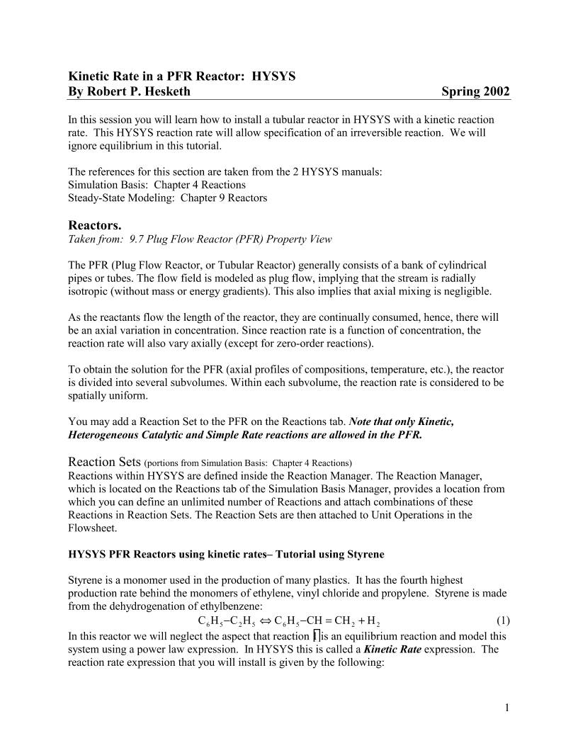
 2
 


















−×−=
T
pr EBEB
K mol
cal1.987
molcal21708exp
s kPaL
EB mol1024.4
reactor
3  (2) 
Notice that the reaction rate has units and that the concentration term is partial pressure with 
units of kPa. 
 
 
Procedure to Install a Kinetic Reaction Rate: 
 
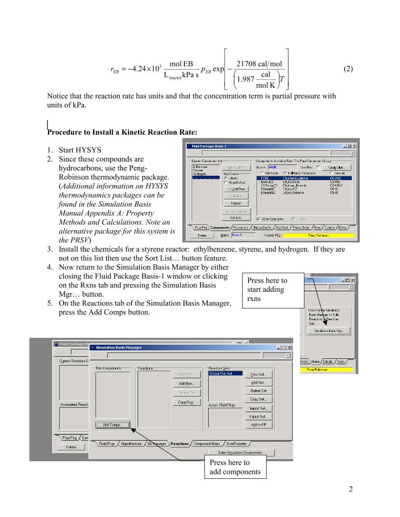
1. Start HYSYS 
2. Since these compounds are 
hydrocarbons, use the Peng-
Robinson thermodynamic package.  
(Additional information on HYSYS 
thermodynamics packages can be 
found in the Simulation Basis 
Manual Appendix A: Property 
Methods and Calculations. Note an 
alternative package for this system is 
the PRSV)  
3. Install the chemicals for a styrene reactor:  ethylbenzene, styrene, and hydrogen.  If they are 
not on this list then use the Sort List… button feature. 
4. Now return to the Simulation Basis Manager by either 
closing the Fluid Package Basis-1 window or clicking 
on the Rxns tab and pressing the Simulation Basis 
Mgr… button.  
5. On the Reactions tab of the Simulation Basis Manager, 
press the Add Comps button.
Press here to 
start adding 
rxns 
Press here to 
add components
 3
 
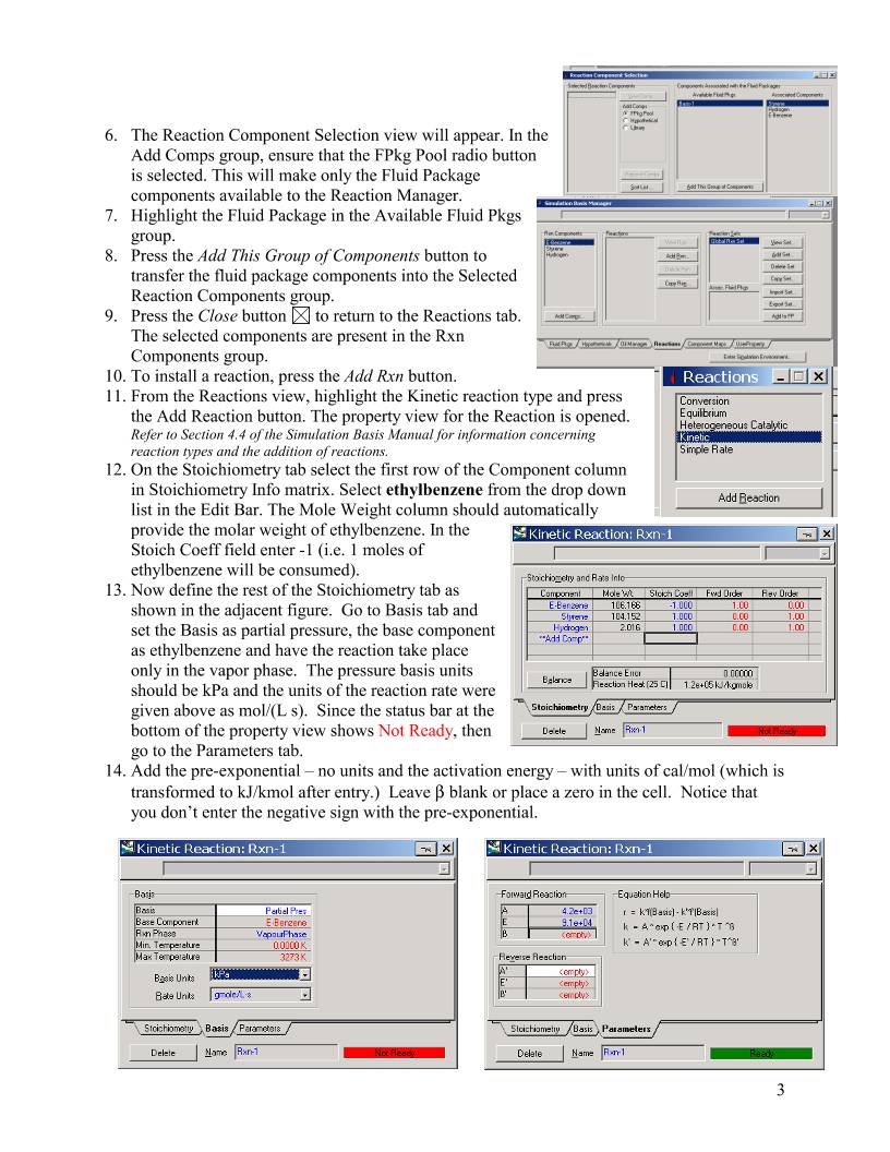
6. The Reaction Component Selection view will appear. In the 
Add Comps group, ensure that the FPkg Pool radio button 
is selected. This will make only the Fluid Package 
components available to the Reaction Manager. 
7. Highlight the Fluid Package in the Available Fluid Pkgs 
group.  
8. Press the Add This Group of Components button to 
transfer the fluid package components into the Selected 
Reaction Components group. 
9. Press the Close button  to return to the Reactions tab. 
The selected components are present in the Rxn 
Components group.  
10. To install a reaction, press the Add Rxn button.  
11. From the Reactions view, highlight the Kinetic reaction type and press 
the Add Reaction button. The property view for the Reaction is opened.  
Refer to Section 4.4 of the Simulation Basis Manual for information concerning 
reaction types and the addition of reactions.  
12. On the Stoichiometry tab select the first row of the Component column 
in Stoichiometry Info matrix. Select ethylbenzene from the drop down 
list in the Edit Bar. The Mole Weight column should automatically 
provide the molar weight of ethylbenzene. In the 
Stoich Coeff field enter -1 (i.e. 1 moles of 
ethylbenzene will be consumed).  
13. Now define the rest of the Stoichiometry tab as 
shown in the adjacent figure.  Go to Basis tab and 
set the Basis as partial pressure, the base component 
as ethylbenzene and have the reaction take place 
only in the vapor phase.  The pressure basis units 
should be kPa and the units of the reaction rate were 
given above as mol/(L s).  Since the status bar at the 
bottom of the property view shows Not Ready, then 
go to the Parameters tab.    
14. Add the pre-exponential – no units and the activation energy – with units of cal/mol (which is 
transformed to kJ/kmol after entry.)  Leave β blank or place a zero in the cell.  Notice that 
you don’t enter the negative sign with the pre-exponential.  
 4
Enter Simulation Environment 
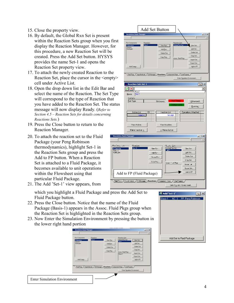
15. Close the property view.  
16. By default, the Global Rxn Set is present 
within the Reaction Sets group when you first 
display the Reaction Manager. However, for 
this procedure, a new Reaction Set will be 
created. Press the Add Set button. HYSYS 
provides the name Set-1 and opens the 
Reaction Set property view.  
17. To attach the newly created Reaction to the 
Reaction Set, place the cursor in the  
cell under Active List.  
18. Open the drop down list in the Edit Bar and 
select the name of the Reaction. The Set Type 
will correspond to the type of Reaction that 
you have added to the Reaction Set. The status 
message will now display Ready. (Refer to 
Section 4.5 – Reaction Sets for details concerning 
Reactions Sets.) 
19. Press the Close button to return to the 
Reaction Manager. 
20. To attach the reaction set to the Fluid 
Package (your Peng Robinson 
thermodynamics), highlight Set-1 in 
the Reaction Sets group and press the 
Add to FP button. When a Reaction 
Set is attached to a Fluid Package, it 
becomes available to unit operations 
within the Flowsheet using that 
particular Fluid Package.  
21. The Add ’Set-1’ view appears, from 
which you highlight a Fluid Package and press the Add Set to 
Fluid Package button.  
22. Press the Close button. Notice that the name of the Fluid 
Package (Basis-1) appears in the Assoc. Fluid Pkgs group when 
the Reaction Set is highlighted in the Reaction Sets group. 
23. Now Enter the Simulation Environment by pressing the button in 
the lower right hand portion  
 
Add Set Button 
Add to FP (Fluid Package)
 5
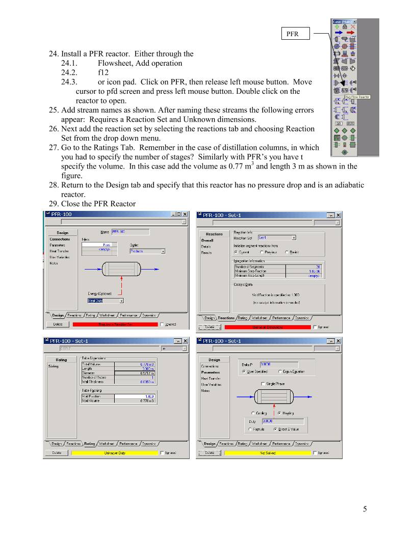
24. Install a PFR reactor.  Either through the 
24.1. Flowsheet, Add operation 
24.2. f12 
24.3. or icon pad.  Click on PFR, then release left mouse button.  Move 
cursor to pfd screen and press left mouse button. Double click on the 
reactor to open.  
25. Add stream names as shown. After naming these streams the following errors 
appear:  Requires a Reaction Set and Unknown dimensions. 
26. Next add the reaction set by selecting the reactions tab and choosing Reaction 
Set from the drop down menu.  
27. Go to the Ratings Tab.  Remember in the case of distillation columns, in which 
you had to specify the number of stages?  Similarly with PFR’s you have t 
specify the volume.  In this case add the volume as 0.77 m3 and length 3 m as shown in the 
figure.   
28. Return to the Design tab and specify that this reactor has no pressure drop and is an adiabatic 
reactor. 
29. Close the PFR Reactor
PFR 
 6
 
30. Open the workbook 
 
31. Now add a feed composition of pure ethylbenzene at 152.2 gmol/s, 880 K, 1.378 bar.  
Remember you can type the variable press the space bar and type or select the units. 
32. Isn’t it strange that you can’t see the molar flowrate in the composition window?  Let’s add 
the molar flowrates to the workbook windows.  Go to Workbook setup. 
33. Press the Add button on the right side 
34. Select Component Molar Flow and then press the All radio button.  
35. To change the units of the variables go to Tools, 
preferences 
Workbook 
Add Button
Comp 
Molar 
Flow
Give it a new name 
such as 
Compositions
 7
36. Then either bring in a previously named preference set or go to the variables tab and clone 
the SI set and give this new set a name.   
37. Change the component molar flowrate units from kmol/hr to gmol/s. 
38. Change the Flow units from kmol/hr to gmol/s 
39. Next change the Energy from kJ/hr to kJ/s. 
40. Save preference set as well as the case.  Remember that you need to open this preference set 
every time you use this case. 
 
41. Notice that the reactor has converged after you added the conditions of the feed stream. 
42. To run an isothermal reactor you need to delete the duty that was specified (in blue) and 
specify the outlet temperature.  Try it!  Isn’t that easy! 
43. Examine the output in the reactor screens by opening the reactor.  Go to the Performance tab 
and make a plot of the composition profile.  Notice that you will have to bring the 
compositions into the plot. 
 
POLYMATH and Hand Calculations 
44. Now we will look at verifying what is going on in HYSYS.  Notice that HYSYS is a black 
box calculation.  You can’t see what it is doing.  Reading the help files will give an 
indication on how it is integrating the reactor.  To fully understand the PFR let’s go to some 
hand calculations given on the following page. 


 8
45. Construct a POLYMATH program to give the following: 
POLYMATH Results 
Styrene Kinetic Rate Model 02-20-2002,   Rev5.1.230  
 
Calculated values of the DEQ variables 
 
 Variable initial value minimal value maximal value final value 
 V 0 0 770 770  
 FEB 152.2 0.2295141 152.2 0.2295141 
 FS 0 0 151.97049 151.97049 
 FH 0 0 151.97049 151.97049 
 FT 152.2 152.2 304.17049 304.17049 
 P 137.8 137.8 137.8 137.8  
 T 880 880 880 880  
 k 0.0172065 0.0172065 0.0172065 0.0172065 
 pEB 137.8 0.103978 137.8 0.103978  
 rEB -2.3710547 -2.3710547 -0.0017891 -0.0017891 
 
ODE Report (RKF45) 
 
 Differential equations as entered by the user 
[1] d(FEB)/d(V) = rEB 
[2] d(FS)/d(V) = -rEB 
[3] d(FH)/d(V) = -rEB 
 
 Explicit equations as entered by the user 
[1] FT = FEB+FS+FH 
[2] P = 137.8 
[3] T = 880 
[4] k = 4.24e3*exp(-21708/1.987/T) 
[5] pEB = FEB/FT*P 
[6] rEB = -k*pEB 
 
 Comments 
[9] P = 137.8 
kPa  
 
 Independent variable  
variable name : V 
initial value : 0 
final value : 770 
 
 Precision  
Step size guess. h = 0.000001 
Truncation error tolerance. eps = 0.000001 
 
 General 
number of differential equations: 3 
number of explicit equations: 6 
Data file: C:\ACdrive\Courses Jan 2002\Reaction Engineering\Lectures&Examples\styrene\styrene kinetic rate 
model.pol 
 
46. Now let’s compare this solution with that given in HYSYS.  Notice that the product flowrates 
of ethylbenzene from POLYMATH is 0.23 mol/s and from HYSYS is 0.55 mol/s.  Why is 
there a difference? 
 9
47. Increasing the number of segments used in the 
integration can reduce the HYSYS product 
flowrate of ethylbenzene.  Go to the following 
screen and change the number of segments and 
observe the effect on the product flowrate of 
ethylbenzene.   
48. Notice that if you increase the number of 
segments, then it will take longer to solve this 
problem.  This could be important when using a 
reactor in a complex chemical plant simulation – 
in you senior year! 
49. Now examine the following screens:  
Notice all 
significant 
digits are 
given 
 10
 
50. Make a plot of the molar flowrates within the PFR.  
Go to the Performance tab and click on composition.   
 
At the end of this exercise submit 4 printouts (5 pages 
total).   
 
1) From a word document printout the following (2 
pages):  (Paste all of your results into one word 
document.)  Make the following plots from your Conversion 
reactor simulation:   
a) The effect of inlet temperature on the conversion 
of ethylbenzene for an adiabatic reactor.  . 
b) The effect of reactor temperature on the conversion of ethylbenzene for an isothermal 
reactor.  Hint:  you can do this using the Databook.  Create a spreadsheet that you can 
import the feed temperature to a cell B1, then export this temperature from a formula in 
cell B2 to the product stream.  See figures on this page for help.  
c) POLYMATH program 
2) On a separate sheet printout the Reaction Summary Printout (See Below for instructions) 
3) On a separate sheet printout the Reactor Summary Printout 
 11
 
Reaction Summary 
1. Go back to the simulation Basis 
Manager by clicking on the 
Erlenmeyer flask.  
2. View the reaction  
3. Remove the pushpin 
4. Select File Print and use the 
preview feature to see the 
following:  
5. Print 
 
Reactor Summary: 
Double click on reactor  
Undo pushpin 
Select Print from main 
menu 
Then select the 
Datablock(s) shown in the 
Select Datablock(s) to Print 
for PFR figure: 
 
Workbook 
Select workbook and print. 
Simulation 
Basis 
Manager 
 12
 
 13