Multiple Reactions.pdf
- 文件大小: 1.51MB
- 文件类型: pdf
- 上传日期: 2025-08-23
- 下载次数: 0
概要信息:
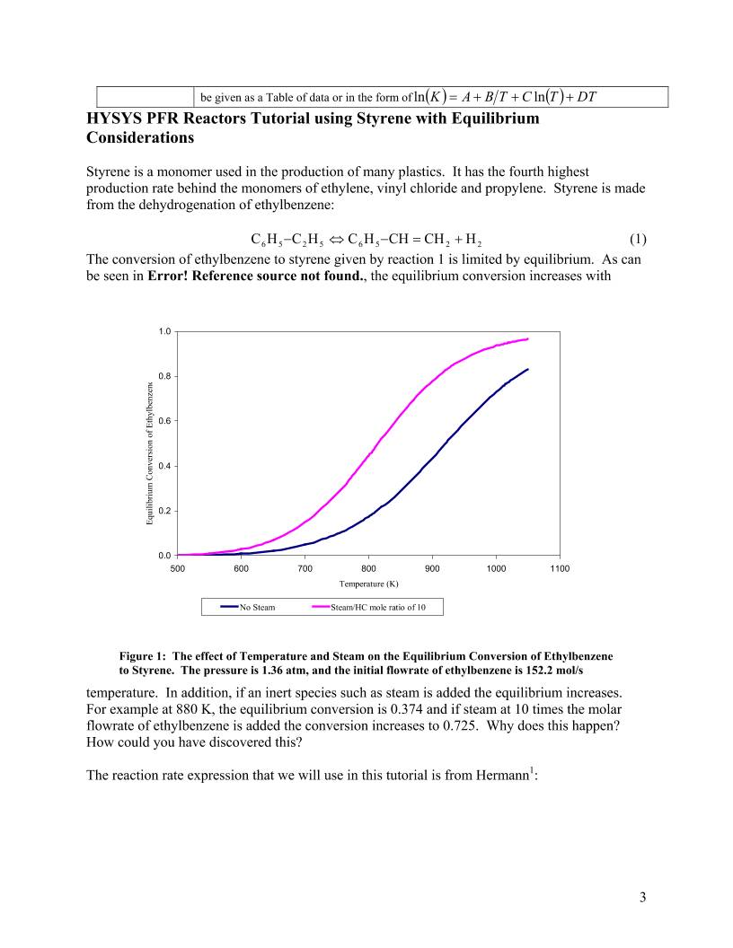
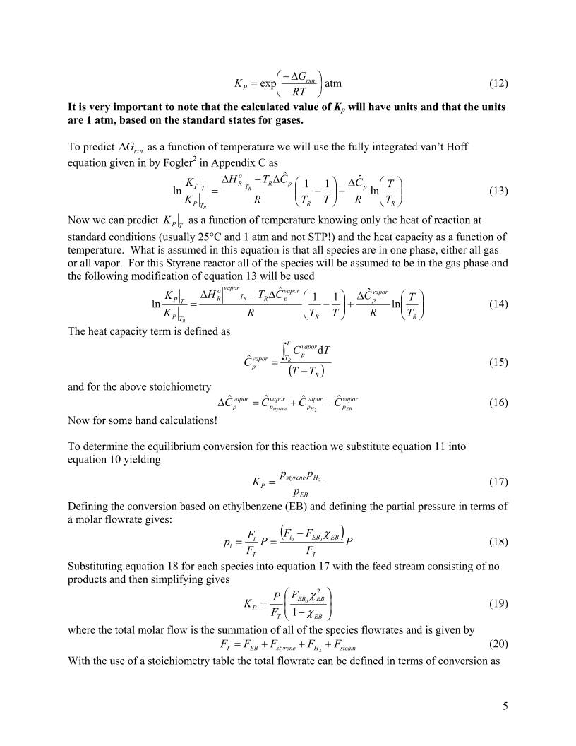
Equilibrium Constant in a Reaction rate in a PFR Reactors: HYSYS By Robert P. Hesketh Spring 2003 In this session you will learn how to use equilibrium constants within a reaction rate expression in HYSYS. You will use the following HYSYS reactors • simple reaction rate expression in a PFR • equilibrium reaction rate in an Equilibrium Reactor • Gibbs reactor. In addition to learning how to use these reactors you will be introduced to the following HYSYS tools: • Adjust Unit Operation • Use of Databook to make 3-D figures • Define a new stream from an existing stream • Investigate the Temperature Independent Properties • Clone a Chemical Species to alter temperature dependent chemical properties Table of Contents Reactor Types in HYSYS ............................................................................................................... 1 1) CSTR model reactors – Well Mixed Tank-Type.................................................................... 1 2) Plug Flow Reactor: Simple Rate, Heterogeneous Catalytic, Kinetic .................................... 2 Reaction Sets (portions from Simulation Basis: Chapter 5 Reactions) ......................................... 2 Summary of Reactions in HYSYS.............................................................................................. 2 HYSYS PFR Reactors Tutorial using Styrene with Equilibrium Considerations .......................... 3 Equilibrium - Theory .................................................................................................................. 4 Hand Calculations for Keq.......................................................................................................... 6 Using the Adjust Unit Operation .............................................................................................. 15 Examine Equilibrium Results at Large Reactor Volumes ........................................................ 16 Equilibrium Reactor...................................................................................................................... 20 Minimization of Gibbs Free Energy ......................................................................................... 24 Gibbs Reactor................................................................................................................................ 25 Submission:................................................................................................................................... 26 The references for this section are taken from the 2 HYSYS manuals: Simulation Basis: Chapter 5 Reactions Operations Guide: Chapter 9 Reactors Reactor Types in HYSYS 1) CSTR model reactors – Well Mixed Tank-Type HYSYS Reactor Name Reaction Types (See above) Conversion Reactor Conversion ( ) 2 210% TCTCCX ++= CSTR Simple Rate, Heterogeneous Catalytic, Kinetic Equilibrium Reactor ( )TfKeq = ; equilibrium based on reaction stoichiometry. predicted from Gibbs Free Energy eqK eqK specified as a constant or from a table of values Gibbs minimization of Gibbs free energy of all specified components, 1 option 1) no the reaction stoichiometry is required option 2) reaction stoichiometry is given 2) Plug Flow Reactor: Simple Rate, Heterogeneous Catalytic, Kinetic Taken from: 9.3 Plug Flow Reactor (PFR) The PFR (Plug Flow Reactor, or Tubular Reactor) generally consists of a bank of cylindrical pipes or tubes. The flow field is modeled as plug flow, implying that the stream is radially isotropic (without mass or energy gradients). This also implies that axial mixing is negligible. As the reactants flow the length of the reactor, they are continually consumed, hence, there will be an axial variation in concentration. Since reaction rate is a function of concentration, the reaction rate will also vary axially (except for zero-order reactions). To obtain the solution for the PFR (axial profiles of compositions, temperature, etc.), the reactor is divided into several subvolumes. Within each subvolume, the reaction rate is considered to be spatially uniform. You may add a Reaction Set to the PFR on the Reactions tab. Note that only Kinetic, Heterogeneous Catalytic and Simple Rate reactions are allowed in the PFR. Reaction Sets (portions from Simulation Basis: Chapter 5 Reactions) Reactions within HYSYS are defined inside the Reaction Manager. The Reaction Manager, which is located on the Reactions tab of the Simulation Basis Manager, provides a location from which you can define an unlimited number of Reactions and attach combinations of these Reactions in Reaction Sets. The Reaction Sets are then attached to Unit Operations in the Flowsheet. Summary of Reactions in HYSYS Reaction Type Description: Conversion Conversion% ( ) 2 210% TCTCCX ++= Equilibrium ( )TfKeq = ; equilibrium based on reaction stoichiometry. predicted or specified eqK Gibbs minimization of Gibbs free energy of all components Kinetic γϕβα SRrevBAfA CCkCCkr +−= where the reverse rate parameters must be thermodynamically consistent and rate constants are given for both the forward and reverse rate constant by ( )RTEATk n −= exp Heterogeneous Catalytic Yang and Hougen form: ∑+ − =− i ii s S r Rb B a A A CK K CCCCk r γ1 This form includes Langmuir-Hinshelwood, Eley-Rideal and Mars-van Krevelen etc. Simple Rate −−= eq SR BAfA K CCCCkr γϕ βα in which is predicted from equilibrium data. must eqK eqK 2 be given as a Table of data or in the form of ( ) ( ) DTTCTBAK +++= lnln 22 HCH += HYSYS PFR Reactors Tutorial using Styrene with Equilibrium Considerations Styrene is a monomer used in the production of many plastics. It has the fourth highest production rate behind the monomers of ethylene, vinyl chloride and propylene. Styrene is made from the dehydrogenation of ethylbenzene: 565256 CHHCHCHC −⇔− (1) The conversion of ethylbenzene to styrene given by reaction 1 is limited by equilibrium. As can be seen in Error! Reference source not found., the equilibrium conversion increases with temperature. In addition, if an inert species such as steam is added the equilibrium increases. For example at 880 K, the equilibrium conversion is 0.374 and if steam at 10 times the molar flowrate of ethylbenzene is added the conversion increases to 0.725. Why does this happen? How could you have discovered this? 0.0 0.2 0.4 0.6 0.8 1.0 500 600 700 800 900 1000 1100 Temperature (K) Eq ui lib riu m C on ve rs io n of E th yl be nz en e No Steam Steam/HC mole ratio of 10 Figure 1: The effect of Temperature and Steam on the Equilibrium Conversion of Ethylbenzene to Styrene. The pressure is 1.36 atm, and the initial flowrate of ethylbenzene is 152.2 mol/s The reaction rate expression that we will use in this tutorial is from Hermann1: 3 − −×−= − P HStyrene EBEB K pp p T r 2 K mol cal1.987 molcal21874exp kPa sg EB mol10491.7 cat 2 (2) Notice that the reaction rate has units and that the concentration term is partial pressure with units of kPa. HYSYS Reaction rates are given in units of volume of gas phase. For example, to convert from units of kgcat given in equation 3 to the units required by HYSYS given in equation 4, you must use equation 5. 4 [ ] gcats mol k r = (3) [ ] 3 gasms mol =HYSYSr (4) ( ) φ φρ − = 1 cHYSYS rr (5) From the source of the original reaction rate studies1 the properties of the catalyst and reactor are given as: 445.0=φ (6) 3 catcat mkg2146=catρ (7) mm7.4=pD (8) For our rates we have been using the units mol/(L s). Take out a piece of paper and write down the conversion from gcat to HYSYS units. Verify with your neighbor that you have the correct reaction rate expression. Please note that if you change the void fraction in your simulation you will need to also change the reaction rate that is based on your void fraction. Equilibrium - Theory In HYSYS, for most reactions you will need to input the equilibrium constant as a function of temperature. The equilibrium constant is defined by equation as ∆− = RT GK rxnexp (9) for the stoichiometry given by equation 1 the equilibrium constant is defined in terms of activities as EB Hstyrene a aa K 2= (10) for a gas the activity of a species is defined in terms of its fugacity ii i i i i pf f fa γ=== atm 10 (11) where iγ has units of atm-1. Now combining equations 9, 10, and 11 results in the following for our stoichiometry given in equation 1, 4 atmexp ∆− = RT GK rxn P (12) It is very important to note that the calculated value of Kp will have units and that the units are 1 atm, based on the standard states for gases. To predict as a function of temperature we will use the fully integrated van’t Hoff equation given in by Fogler2 in Appendix C as rxnG∆ ∆ + − ∆−∆ = R p R pRT o R TP TP T T R C TTR CTH K K R R ln ˆ11 ˆ ln (13) Now we can predict TPK as a function of temperature knowing only the heat of reaction at standard conditions (usually 25°C and 1 atm and not STP!) and the heat capacity as a function of temperature. What is assumed in this equation is that all species are in one phase, either all gas or all vapor. For this Styrene reactor all of the species will be assumed to be in the gas phase and the following modification of equation 13 will be used ∆ + − ∆−∆ = R vapor p R vapor pRT vaporo R TP TP T T R C TTR CTH K K R R ln ˆ11ˆ ln (14) The heat capacity term is defined as ( )R T T vapor pvapor p TT TC C R − = ∫ d ˆ (15) and for the above stoichiometry (16) vapor p vapor p vapor p vapor p EBHstyrene CCCC ˆˆˆˆ 2 −+=∆ Now for some hand calculations! To determine the equilibrium conversion for this reaction we substitute equation 11 into equation 10 yielding EB Hstyrene P p pp K 2= (17) Defining the conversion based on ethylbenzene (EB) and defining the partial pressure in terms of a molar flowrate gives: ( ) P F FF P F Fp T EBEBi T i i χ 00 − == (18) Substituting equation 18 for each species into equation 17 with the feed stream consisting of no products and then simplifying gives − = EB EBEB T P F F PK χ χ 1 2 0 (19) where the total molar flow is the summation of all of the species flowrates and is given by steamHstyreneEBT FFFFF +++= 2 (20) With the use of a stoichiometry table the total flowrate can be defined in terms of conversion as 5 EBEBsteamEBT FFFF χ 000 ++= (21) Substituting equation 21 into equation 19 gives the following equation ( ) −+ = EB EBEB EBEBT P F FF PK χ χ χ 1 2 0 0 0 (22) The above equation can be solved using the quadratic equation formula and is ( ) ( ) ( )PEB TPPEBsteamPsteamP EB KPF FKKPFFKFK + +++− = 0 000 2 4 0 2 χ (23) There are 2 very important aspects to Styrene reactor operation that can be deduced from equation 19 or 22. Knowing that at a given temperature Kp is a constant then 1. Increasing the total pressure,P, will decrease χEB 2. Increasing the total molar flowrate by adding an inert such as steam will increase χEB The following page gives sample calculations for all of the above. From these sample calculations at a temperature of 880 K the equilibrium constant is 0.221 atm. At an inlet flowrate of 152.2 mol ethylbenzene/s and no steam the conversion is 0.372. At an inlet flowrate of 152.2 mol ethylbenzene/s and a steam flowrate of 10 times the molar flowrate of ethylbenzene the conversion increases to 0.723. Once you have calculated Kp as a function of temperature, then you can enter this data into a table for the reaction rate. Hand Calculations for Keq 6 Procedure to Install a Reaction Rate with an Equilibrium Constant – Simple Reaction Rates 1. Start HYSYS 2. Since these compounds are hydrocarbons, use the Peng- Robinson thermodynamic package. (Additional information on HYSYS thermodynamics packages can be found in the Simulation Basis Manual Appendix A: Property Methods and Calculatio Note an alternative package for this system is the ns. 3. n this list then use the Sort List… button 4. window and selecting Basis Manager from 6. ss asis Manual for 7. . In the Stoich Coeff field enter -1 (i.e. 1 moles of ethylbenzene will be define the rest of the Stoichiometry tab as shown 9. Press here to start adding rxns PRSV) Install the chemicals for a styrene reactor: ethylbenzene, styrene, hydrogen and water. If they are not o feature. Now return to the Simulation Basis Manager by selecting the Rxns tab and pressing the Simulation Basis Mgr… button or close the Fluid Package Basis-1 the menu. 5. To install a reaction, press the Add Rxn button. From the Reactions view, highlight the Simple Rate reaction type and pre the Add Reaction button. Refer to Section 4.4 of the Simulation B information concerning reaction types and the addition of reactions. On the Stoichiometry tab select the first row of the Component column in Stoichiometry Info matrix. Select ethylbenzene from the drop down list in the Edit Bar. The Mole Weight column should automatically provide the molar weight of ethylbenzene consumed). 8. Now in the adjacent figure. Go to Basis tab and set the Basis as partial pressure, the base component as ethylbenzene and 9 have the reaction take place only in the vapor phase. 10. The pressure basis units should be atm and the units of the reaction rate given by equation 24 11. b and enter the activation energy from equation 2 is is mol/(L s). Since the status bar at the bottom of the property view shows Not Ready, then go to the Parameters tab. Next go to the Parameters ta molcalEa 21874= . Convert the pre-exponential from units of kPa to have unit n be made later in this tutorial. : (1kg 2146g10mol 3 2 −− s of atm so that a comparison ca ) atm sgcat mol20315 atm Pa1001325.1 Pa1000 kPa1 kPa sL mol5.200 L 10 m 1 m 0.445 m m m 445.0 mkgkPa sgcat 10491.7 5 gas gas 3 3 gas 3 gas 3 R 3 R 3 cat 3 cat cat cat cat = × = ×=A (24) 12. Leave β blank or place a zero in the cell. Notice that you don’t enter the negative sign with 13. your equilibrium constant values, with units of atm, using the equation the pre-exponential. Now you must regress ( ) ( ) DTTCTBAK +++= lnln (25) 14. Below is the data table that is produced using the integrated van’t Hoff expression shown in 10 7.92 550 1.10E-05 600 9.99E-05 650 6.46E-04 700 3.20E-03 750 0.013 775 0.024 800 0.043 810 0.054 820 0.067 830 0.082 840 0.101 850 0.124 860 0.151 870 0.183 880 0.221 890 0.266 900 0.318 910 0.379 920 0.450 930 0.532 950 0.736 970 1.003 990 1.348 010 1.791 1030 2.351 1050 3.051 equation 14. These data can either be regressed using Microsoft Excel’s multiple linear Regression or a nonlinear regression program such as polymath. Make sure that the units of Kp are the same as your basis units. T (K) Kp (atm) 500 E-07 1 Enter Simulation Environment Add to FP (Fluid Package) 15. The results of the regression of the predicted K values with the HYSYS equilibrium constant equation 25 are shown in the adjacent table. Add these constants to the Simple Rate window. Make sure you add many significant digits! 16. Name this reaction from Rxn-1 to Hermann eq. Close the Simple Rate Window after observing the green Ready symbol. Coefficients A’ -13.2117277 B’ -13122.4699 C’ 4.353627619 D’ -0.00329709 17. By default, the Global Rxn Set is present within the Reaction Sets group when you first display the Reaction Manager. However, for this procedure, a new Reaction Set will be created. Press the Add Set button. HYSYS provides the name Set-1 and opens the Reaction Set property view. 18. To attach the newly created Reaction to the Reaction Set, place the cursor in thecell under Active List. 19. Open the drop down list in the Edit Bar and select the name of the Reaction. The Set Type will correspond to the type of Reaction that you have added to the Reaction Set. The status message will now display Ready. (Refer to Section 4.5 – Reaction Sets for details concerning Reactions Sets.) 20. Press the Close button to return to the Reaction Manager. 21. To attach the reaction set to the Fluid Package (your Peng Robinson thermodynamics), highlight Set-1 in the Reaction Sets group and press the Add to FP button. When a Reaction Set is 11 attached to a Fluid Package, it becomes available to unit operations within the Flowsheet using that particular Fluid Package. 22. The Add ’Set-1’ view appears, from which you highlight a Fluid Package and press the Add Set to Fluid Package button. 23. Press the Close button. Notice that the name of the Fluid Package (Basis-1) appears in the Assoc. Fluid Pkgs group when the Reaction Set is highlighted in the Reaction Sets group. PFR 24. Now Enter the Simulation Environment by pressing the button in the lower right hand portion 25. Install a PFR reactor. Either through the 25.1. Flowsheet, Add operation 25.2. f12 25.3. or icon pad. Click on PFR, then release left mouse button. Move cursor to pfd screen and press left mouse button. Double click on the reactor to open. 26. Add stream names as shown. 27. Next go to the Parameters portion of the Design window. Click on the radio button next to the pressure drop calculation by the Ergun equation. 28. Next add the reaction set by selecting the reactions tab and choosing Reaction Set from the drop down menu. 29. Go to the Rating Tab. Remember in the case of distillation columns, in which you had to specify the number of stages? Similarly with PFR’s you have to specify the volume. In this case add the volume as 250 m3, 7 m length, and a void fraction of 0.445 as shown in the figure. 12 30. Return to the Reactions tab and modify the specifications for your catalyst to the density and particle size given on page 4. 31. Go to the Design Tab and select heat transfer. For this tutorial we will have an isothermal reactor so leave this unspecified. 32. Close the PFR Reactor 13 33. Open the workbook 34. Isn’t it strange that you can’t see the molar flowrate in the composition window? Do you have a composition tab? Let’s add the molar flowrates to the workbook windows. Go to Workbook setup either by right clicking on a tab or choosing workbook setup form the menu. 35. If you don’t have a composition tab then, press the Add button on the left side and add a material stream and rename it Compositions. 36. In the Compositions workbook tab, select Component Molar Flow and then press the All radio button. 37. To change the units of the variables go to Tools, preferences 38. Then either bring in a previously named preference set or go to the variables tab and clone the SI set and give this new set a name. Button 39. Change the component molar flowrate units from kmol/hr to gmol/s. 40. Change the Flow units from kmol/hr to gmol/s Give it a new name such as Compositions41. Next change the Energy from kJ/hr to kJ/s. Add 42. Save preference set as well as the case. Remember that you need to open this preference set every time you use this case. Workbook Comp Molar Flow 14 Back to the Simulation 43. Now add a feed composition of pure ethylbenzene at 152.2 gmol/s, 1522 gmol/s of water, 880 K, and 1.378 bar. Then set the outlet temperature to 880K to obtain an isothermal reactor. Remember you can type the variable and then press the space bar and type or select the units. 44. No the reactor should solve for the outlet concentrations. Take a note of the pressure drop in the Design Parameters menu. I got a pressure drop of 86.38 kPa. Now change the length of the reactor to 8 m. If you get the above message then your reactor has not converged and you need to make adjustments to get your reactor to converge (e.g. the product stream is empty!) Now it is your task to reduce the pressure drop to an acceptable level. What do you need to alter? Refer to the Ergun Equation given by ( ) + − − −= G DD GP pp 75.111501 dz d 3 µφ φ φ ρ (26) Using the Adjust Unit Operation Adjust 45. Obtain a solution that will meet the following pressure drop specification One way of doing this quickly is to use the adjust function. Go to Flowsheet, Add operation (or press f12 or the green A in a diamond on the object palette. 01.0 PP ≤∆ 46. Now select the adjusted variable as the tube length and the target variable as the Pressure Drop. Set the pressure drop to 13.78 kPa (exactly 10% of P0). 15 47. Next go to the Parameters tab and set the tolerance, step size and maximum iterations. If you have problems you can always press the Ignored button in the lower right hand corner of the page, then go back to the reactor and change the values by hand. If it stops, it may ask you if you want to continue. Answer yes. You can watch the stepping progress by going to the monitor tab. 48. Try this again, but this time get your pressure drop to 1% of P0. 49. Now turn this Adjust unit off by clicking on the ignored button. Examine Equilibrium Results at Large Reactor Volumes 50. You equilibrium conversion should be around 72.6%. Comparing this to the hand calculated results for a steam to hydrocarbon molar ratio of 10 is 72.3% at 880 and 137.8kPa. 51. Set your pressure drop to zero by turning off the Ergun equation in the Reactor, Design Tab, Parameters option. Set the pressure drop to zero. The conversion is now 72.5%! Which again is very close to your hand calculations. Ignored button 16 Now set the feed flowrate of steam to zero. You should get a conversion of 37.4%. This again is what your spreadsheet calculation shows for 880K and 137.8 kPa. 52. How do you know that you have reached the equilibrium conversion that is limiting this reaction? M a plot of the molar flowrate of ethylbenzene using the tool in the performance tab and com option of the reactor. ake position 53. Next, make a plot of conversion as a function of both reactor temperature and pressure. Becareful how you set up this databook. I had 943 data states by varying both and . Remember that you have to setup a workbook so that you only need to specify the temperature in one cell. I would suggest that you add a spreadsheet to keep all of your calculations in one area. kPaPkPa 500100 ≤≤ KTK 1050500 ≤≤ 17 54. Now make a plot of the effect of steam flow and temperature on conversion. You will need to add a new feed stream to the reactor. 54.1. Make your Feed stream have only 152.2 mol of ethylbenzene per second. 18 54.2. Make a second feed steam called water have a flow of 0 mol/s. Create a second cell in your spreadsheet that you can export the temperature to the Water feed stream temperature as well as the outlet stream, Product, to make the reactor isothermal and to the. Notice that you had to specify one cell for each export. 54.3. Reorder your workbook by going into the menu for the workbook and choosing order/hide/reveal Objects. Then put the water stream next to the feed stream. 54.4. In the Data book bring in the following variables so that the water molar flow will be considered an independent variable. (don’t do the number of states in these examples!) 19 General Reactors Equilibrium Reactors Equilibrium Reactor 55. Now we will install a second reactor that only contains an equilibrium reaction. Use either the object palette or the Flowsheet, Add Operation, Equilibrium Reactor. 56. Label the streams as shown 57. Notice that in Red is a warning that it needs a reaction set. Let’s see if it likes the one we already have. Pull in the reaction being used by the PFR. Whoops! It didn’t like this one! Equilibrium reactors can only have equilibrium reactions. We will have to create a new one. 58. Click on the Erlenmeyer flask or choose Simulation, Enter Basis Environment. 59. Add a new reaction. 60. Go to the Library tab and choose the library reaction. Wow it was in there all the time! 20 61. Look at the Keq page.A plot of the data given in the HYSYS table and the equation that HYSYS uses to fit the data is given below. This comparison shows that the hand calculations and the HYSYS stored values are in good agreement with each other in the temperature range of . Above 920 K the v of K begin to deviate from each other. K 920500 ≤≤ T alues 62. Attach the equilibrium reaction to a new 11. or 63. Return to the reactor using the green arrow ou t. t 64. the Go back to pfd or leave basis reaction set starting with step 17 on page (The step 17 is a hyperlink and is active in adobe.) Title the new set Equilibrium React Set. When finished return to the step 63. environment and bring in the new reaction set to the equilibrium reactor. Now you see why y need in some cases more than one reaction se Another reason is that you may want one se of reactions for a dehydrogenation reactor and then a separate set for an oxidation reactor. Bring in the equilibrium reaction set into reactor 21 65. Now specify the EQ Feed stream to be identical to the Feed stream. This can be done by double clicking on the EQ Feed title or name. And then choosing the Define from Other Stream… option. 66. Define the temperature of one outlet stream to be equal to the feed. Examine the following 2 conditions from your PFR simulations at 880 K and 1.378 bar with: Cases HYSYS Library Hand Calculations 0 2.152 0 = = steam EB F smolF 2595.0 03.40 = = K χ 221.0 4.37 = = K χ smolF smolF steam EB 1522 2.152 0 = = 2595.0 95.74 = = K χ 2595.0 5.72 = = K χ Result for no steam flow 22 67. Now add the values from your hand calculation into the equilibrium reactor. Go to view reaction and enter these values within the reactor’s reaction tab. Within the equilibrium reaction choose the basis tab and select the Ln(Keq) Equation: Coefficients A -13.2117277 B -13122.4699 C 4.353627619 D -0.00329709 68. Next enter the following table of coefficients for this equation 69. Now rerun the above cases. This will predict the PFR equilibrium values given in the table below. Cases HYSYS Library Hand Calculations Regression from Hand Calculations 0 2.152 0 = = steam EB F smolF 2595.0 03.40 = = K χ 221.0 4.37 = = K χ 221.0 4.37 = = K χ smolF smolF steam EB 1522 2.152 0 = = 2595.0 95.74 = = K χ 221.0 5.72 = = K χ 221.0 5.72 = = K χ Notice that with the PFR you need a large volume or mass of catalyst to achieve these equilibrium values. You previously tried this with your PFR and you came close to these above values. In step 51 on page 16 your PFR values were 37.42 and 72.5%. 70. Which values are correct? Since, no reference is given by HYSYS to the library reaction and you know the source of the hand calculations3 you should trust your hand calculations. 23 Minimization of Gibbs Free Energy 71. Go back to the reaction screen and choose the Gibbs Free Energy radio button. 72. You get a conversion of 74.80 and K=0.2569. In an older version of HYSYS you mistakenly got 100% conversion. In the Gibbs Free energy minimization, the equilibrium constant is determined from the Ideal Gas Gibbs Free Energy Coefficients in the HYSYS library. 73. ne th 73.1 basis 73.3 styrene and view the mpo 73.4 e s l e! to investigate what it is doing. Exami ese values. . Enter the environment. 73.2. View the property package . Select co nent . Choose the temperatur dependent tab: Tdep. In the current version of HYSYS the temperature dependent propertie of Styrene are given for all the ideal gas properties. In an old version of HYSYS, only one coefficient was given for the Idea Gas Gibbs Free Energy. In this case the Ideal Gas Gibbs Free Energy was a constant and independent of temperatur This was incorrect. In the previous version new values were obtained from Aaron Pollock of Hyprotech Technical Support.4 This is a clear example of why you need critically examine the results produced by a process simulator! You always need to Old Version: 100% 24 View Component Old Version G=constant 74. To modify properties you must create a hypothetical component that can either be a clone of ations Gib reactor called a Gibbs Reactor 76. Put in the conditions given in step 65 on page 22 nergy results. The only difference for this reactor is a current chemical or an entirely new hypothetical component in which the properties are estimated using standard and proprietary methods. See the Adobe pdf help manual: Simulation Guide Chapter 3. (go to the link in the reaction engineering homepage) Many of the estim are based on the UNIFAC structure which is described in section 3.4.3 of that chapter. bs Reactor 75. Now install a 3rd and label the streams and define the feed and outlet temperature of the streams. above. Notice that the same result as an equilibrium reactor using the gibbs free e that you did not need to specify the stoichiometry of the reaction. 25 Submission: At the end of this exercise submit 1) The following graphs from PFR a) the effect of temperature and pressure on equilibrium conversion (see step 53) b) the effect of the molar flow of steam and temperature on equilibrium conversion at a fixed pressure and ethylbenzene flowrate (see step 54). c) Short summary of the effect of T, P and steam flow on equilibrium conversion. 2) Pfd of the three reactors 26 References: 1 Hermann, Ch.; Quicker, P.; Dittmeyer, R., “Mathematical simulation of catalytic dehydrogenation of ethylbenzene to styrene in a composite palladium membrane reactor.” J. Membr. Sci. (1997), 136(1-2), 161-172. 2 Fogler, H. S. Elements of Chemical Reaction Engineering, 3rd Ed., by, Prentice Hall PTR, Englewood Cliffs, NJ (1999). 3 "Thermodynamics Source Database" by Thermodynamics Research Center, NIST Boulder Laboratories, M. Frenkel director, in NIST Chemistry WebBook, NIST Standard Reference Database Number 69, Eds. P.J. Linstrom and W.G. Mallard, July 2001, National Institute of Standards and Technology, Gaithersburg MD, 20899 (http://webbook.nist.gov). 4 Yaws, C.L. and Chiang, P.Y., "Find Favorable Reactions Faster", Hydrocarbon Processing, November 1988, pg 81-84.
缩略图:
高速下载:
正在进行安全检测...
点击后进入安全下载页,再进行实际下载。下载链接有效期 24 小时,过期会自动刷新。
下载说明:
- 文件描述:Multiple Reactions.pdf,可用于在线分享与下载使用。
- 文件分类:文档资料
- 用途建议:适用于资料分享、学习交流、办公协作。
- 适合人群:学生、教师、办公人员、项目协作团队。
- 适配系统:Windows、macOS、Android、iOS 均可下载访问。